Please switch off AdBlock for this webside to display it correctly (there are no ads here).
Tauc-Lorentz dispersion model
modelname
Tauc-Lorentz|TL
Imaginary part of complex dielectric function is described by four parameters \(E_\mathrm{g}, N_1, E_1, B_1\).
The TL model can be calculated by five different parametrizations, see attributes
CC,
JM,
DF1,
ASF and
DF2.
In the case that no attribute is chosen, the another four parameters are generated, i.e.
\(f_{\rm JM}\), \(f_{\rm CC}\), \(f_{\rm DF1}\), \(f_{\rm DF2}\).
Dielectric function is then calculated as linear combination of the all version of Tauc-Lorent model:
$$
\begin{array}{l}
\hat\varepsilon(E) = 1 + f_{\rm DF2} \ \hat\chi_{\rm DF2}(E) + (1-f_{\rm DF2}) \\
\times \Bigg( f_{\rm CC} \ \hat\chi_{\rm CC}(E) + (1-f_{\rm CC}) \Big( f_{\rm DF1} \ \hat\chi_{\rm DF1}(E) + (1-f_{\rm DF1})
\big( f_{\rm JM} \hat\chi_{\rm JM}(E) + (1-f_{\rm JM}) \, \hat\chi_{\rm ASF}(E) \big)\Big) \Bigg)
\end{array}
$$
where \(\hat\chi\) are corresponding susceptibilities.
attributes
-
CC - Campi-Corriasso version of TL model:
$$
\begin{array}{lcl}
\displaystyle
\varepsilon_\mathrm{i} = \frac{2}{\pi} \frac{N_1 B_1 (E-E_\mathrm{g})^2}{E(((E-E_\mathrm{g})^2-(E_1-E_\mathrm{g})^2)^2+B_1^2 (E-E_\mathrm{g})^2)} & \mathrm{for} & E > E_\mathrm{g} \\
\varepsilon_\mathrm{i} = 0 & \mathrm{for} & E \leq E_\mathrm{g}
\end{array}
$$
Real part of dielectric function is expressed analyticlally using the Kramers-Kronig relation.
-
JM - Jellison-Modine version of TL model:
$$
\begin{array}{lcl}
\displaystyle
\varepsilon_\mathrm{i} = \frac{N_1(E-E_\mathrm{g})^2}{{\cal C}_\mathrm{N} E ((E^2-E_1^2)^2+B_1^2 E^2)} & \mathrm{for} & E > E_\mathrm{g} \\
\varepsilon_\mathrm{i} = 0 & \mathrm{for} & E \leq E_\mathrm{g}
\end{array}
$$
where \(C_\mathrm{N}\) is normalization constant. Real part of dielectric function is expressed analyticlally using the Kramers-Kronig relation.
-
DF1 - Our first version of TL model:
$$
\begin{array}{lcl}
\displaystyle
\varepsilon_\mathrm{i} = \frac{N_1 (E - E_\mathrm{g})^2}{{\cal C}_\mathrm{N}E^3((E-\sqrt{E_1^2-B_1^2/4})^2+B_1^2/4)} & \mathrm{for} & E > E_\mathrm{g} \\
\varepsilon_\mathrm{i} = 0 & \mathrm{for} & E \leq E_\mathrm{g}
\end{array}
$$
where \(C_\mathrm{N}\) is normalization constant. Real part of dielectric function is expressed analyticlally using the Kramers-Kronig relation.
-
ASF - A.S. Ferlauto at al. version of TL model:
$$
\begin{array}{lcl}
\displaystyle
\varepsilon_\mathrm{i} = \frac{N_1 \, E \, (E-E_\mathrm{g})^2}{{\cal C}_\mathrm{N} ((E-E_\mathrm{g})^2 + E_\mathrm{p}^2) \,
((E^2-E_1^2)^2+B_1^2 E^2)} & \mathrm{for} & E > E_\mathrm{g} \\
\varepsilon_\mathrm{i} = 0 & \mathrm{for} & E \leq E_\mathrm{g}
\end{array}
$$
where \(C_\mathrm{N}\) is normalization constant. This approximation have one extra parameter \(E_\mathrm{p}\),
which influences transition strength below and above peak energy.
Real part of dielectric function is expressed analyticlally using the Kramers-Kronig relation.
-
DF2 - Our second version of TL model:
$$
\begin{array}{lcl}
\displaystyle
\varepsilon_\mathrm{i} = \frac{N_1 (E - E_\mathrm{g})^2}{{\cal C}_\mathrm{N}E((E-E_\mathrm{g})^2 + E_\mathrm{p}^2)((E-\sqrt{E_1^2-B_1^2/4})^2+B_1^2/4)} & \mathrm{for} & E > E_\mathrm{g} \\
\varepsilon_\mathrm{i} = 0 & \mathrm{for} & E \leq E_\mathrm{g}
\end{array}
$$
where \(C_\mathrm{N}\) is normalization constant. Real part of dielectric function is expressed analyticlally using the Kramers-Kronig relation.
-
CJF - Linear combination of CC, JM and DF1 version of TL model:
$$
\hat\varepsilon(E) = 1 + f_{\rm CC} \ \hat\chi_{\rm CC}(E) + (1-f_{\rm CC}) \Big( f_{\rm JM} \ \hat\chi_{\rm JM}(E) + (1-f_{\rm JM}) \, \hat\chi_{\rm DF1}(E) \Big) .
$$
-
number_of_terms - Adds terms and corresponding parameters \(N_2, E_2, B_2, \dots\).
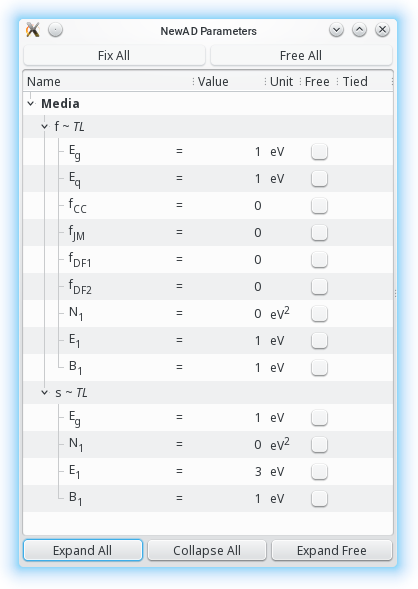
Example
media:
  f = TL
  s = TL:CC
newAD2> par
  Egf = 1          fixed (0,inf) eV
  Eqf = 1          fixed (0,inf) eV
 fCCf = 0          fixed [0,1]
 fJMf = 0          fixed [0,1]
fDF1f = 0          fixed [0,1]
fDF2f = 0          fixed [0,1]
  N1f = 0          fixed [0,inf) eV2
  E1f = 3          fixed (1e-4,inf) eV
  B1f = 1          fixed (1e-4,inf) eV
  Egs = 1          fixed (0,inf) eV
  N1s = 0          fixed [0,inf) eV2
  E1s = 3          fixed (1e-4,inf) eV
  B1s = 1          fixed (1e-4,inf) eV
newAD2>
 |
|